When a Power BI report does not match SQL Server, the fastest way to respond is often to examine the DAX. That’s understandable, particularly when the visual is the first place the wrong number is apparent. It is also a frequent waste of time. A perfectly valid SUM can lead to the wrong business result if the rows hitting the semantic model are already multiplied, filtered differently or loaded at a different grain than the source.

In Power BI Consulting work, the better approach is to view reconciliation as a data-contract problem first, then a calculation problem. The contract should include the reporting period, business grain, expected row count, expected distinct business key count and at least one additive amount that can be validated at each layer.

That principle is illustrated in the small SQL Server example we are using here. The correct source has 18 line rows, 9 orders, 6 customers and $2,825 in net sales for completed orders in the window from January 1, 2026, inclusive through March 1, 2026, exclusive. A deliberate bad one-to-many join blows up the rows to 28 and keeps the distinct order count at 9. Net sales rises to $4,825. The $2,000 difference is a 70.8% overstatement. The DAX can still be totally normal.

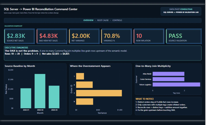
Figure 1: Power BI SQL Reconciliation Command Center

The correct source is still at $2,830. The intentionally bad join is at $4,830. That is a $2,000/70.8% variance.

Resource Toolkit

Separating the evidence from the presentation makes it easier to reproduce the workflow. The companion toolkit for this example has a T-SQL validation script, a correct SQL view at the intended line grain, a deliberately bad join used as a control, a Power Query and DAX reference and two Power BI pages that show the reconciliation and root-cause results.

The dashboard is not the most important thing. It is the set of numbers that each layer needs to be able to reproduce. For this demo, the core contract is 18 rows, 9 unique orders, 6 customers and $2,825 net sales for the right Jan-Feb window. The bad path deliberately gives 28 rows and $4,825 while the 9 distinct orders stay the same. Those values give the developer something to prove or disprove at each stage.

A good rule of thumb is to collect the evidence before you change the model. When a report has been ‘fixed’ in several places at once, it is difficult to determine which change actually fixed the issue. The sequence of troubleshooting is repeatable with one controlled defect and a small set of locked checks.

Problem: Why the Correct DAX Can Still Produce the Wrong Number

Let’s assume we have a sales fact table that should contain one row per OrderLineID. At that grain, it is safe to sum an additive measure such as net sales as long as each business row appears only once.

Now add a CustomerTag table, where a customer can have several tags. If you join sales rows directly to CustomerTag before data gets to Power BI, you might end up repeating each sales row for a customer with multiple tags once for each tag that matches. The database is not necessarily ‘wrong’ in the sense of causing an invalid join. The problem is that the result no longer has the grain that the report expects.

That’s exactly what happens in the demo. The right answer has 18 rows, the wrong path has 28, but both still have 9 different orders. That is a strong diagnostic signal: The row count went up, but a higher-level business key did not.

The size of the problem is such that the defect cannot be dismissed as a harmless duplication of descriptive attributes. Correct net sales is $2,825. The bad result is $4,825. Four orders account for the overstatement: Order 1 is high by $180, Order 4 is high by $380, Order 7 is high by $1,050 and Order 9 is high by $390. Those four differences total the entire $2,000 variance.

This is due to the customer-side pattern. In the test data, Customer 1 has two tag rows, Customer 3 has two and Customer 6 has three. Customers with one tag do not inflate their orders. Customers with many tags do. The largest order variance corresponds to the customer with the highest multiplicity.

That’s a better root cause statement than ‘Power BI is double counting’. The report is not making up rows. In the upstream dataset, there were multiple copies of line-grain facts because a one-to-many descriptive table was joined at the wrong point in the pipeline.

Microsoft guidance for Power BI modeling states that fact tables should be loaded at a consistent grain, and one-to-many relationships should follow a clear dimension-to-fact pattern. A bridge is usually the preferred choice when you want to represent a real many-to-many dimension relationship. The practical implication is simple: Do not flatten a multi-valued descriptive relationship onto an additive fact set unless you intentionally account for the change in grain. 

Solution: Start With the SQL Server Reconciliation Contract

Run a source-side query that returns three types of evidence: Row count, distinct business keys and an additive amount, before getting to Power Query or DAX. This is the trifecta of reconciliation.

A schema-neutral version would look like:

DECLARE @PeriodStart date = ‘2026-01-01’;
DECLARE @NextPeriodStart date = ‘2026-03-01’;
SELECT
    COUNT_BIG(*) AS RowCount,
    COUNT(DISTINCT OrderID) AS DistinctOrders,
    SUM(NetSales) AS NetSales
FROM <correct_line_grain_source>
WHERE OrderStatus = ‘Completed’
  AND OrderDate >= @PeriodStart
  AND OrderDate < @NextPeriodStart;

Replace the placeholder source and column names with the actual schema. In the validated demo, the correct Power BI-facing source is demo.vw_PowerBI_Sales_Correct. The expected contract for this same period is 18 rows, 9 orders and $2,825.

Why all three checks? It is because a total can coincide by chance. The keys might not match, but the row counts might. A distinct-order count can also tie if some lines are missing and others are duplicated. The three checks are more powerful together.

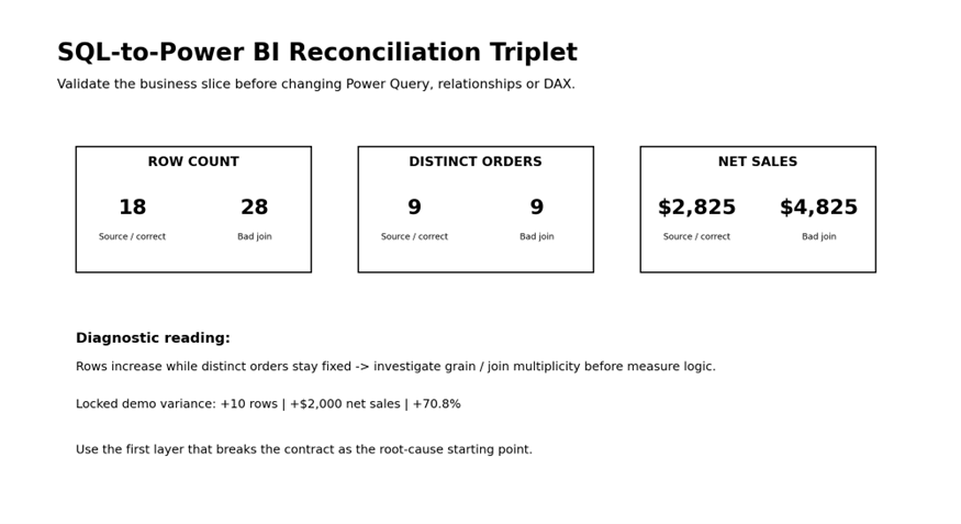
Figure 2: Reconciliation Triplet: Row Count, Distinct Business Keys and Additive Amount Isolate a Grain Problem Before DAX Debugging

The following SQL check should test the fact grain directly:

SELECT
    OrderLineID,
    COUNT_BIG(*) AS Copies
FROM <candidate_result>
GROUP BY OrderLineID
HAVING COUNT_BIG(*) <> 1;

For a source that promises one row per OrderLineID, the above query should return no rows. If it returns duplicate IDs, stop here. Don’t compensate in DAX.

Then reconcile up at the business level above the fact grain. OrderID is useful in this example because the total number of orders remains the same even if the line rows are multiplied. Correct and candidate amounts can be compared to isolate exactly where the financial divergence occurs.

The demo found four inflated orders and no change in the distinct-order count. That quickly reduced the search from “the report total is wrong” to “these four orders were multiplied somewhere below order grain.”

Use Half-Open Date Ranges

Date filters are another frequent cause of SQL and Power BI disagreeing even with the correct row grain. The safest reusable pattern for a bounded period is:

WHERE OrderDate >= @PeriodStart AND OrderDate < @NextPeriodStart

The demo tests this on purpose. The right Jan-Feb window yields $2,825. Include March 1 and the total becomes $3,525. That creates a $700 boundary leak.

If the source column is a datetime and not a pure date, the half-open pattern is even more important. If the data has time values, ‘2026-02-28’ may silently exclude later-in-the-day rows. You don’t have to invent an end-of-day timestamp, because you start the next period.

Trace the First Divergent Grain Before Touching the Semantic Model

Freeze SQL baseline and compare to each downstream layer. The aim is not to show that the final dashboard is wrong. You know that already. You want to find the first place where the contract doesn’t work anymore.

In the test case, the right path is Order Header -> Order Line -> Customer. The bad path extends that chain from Customer to CustomerTag, which multiplies the line-grain rows. That is the first divergent grain.

You can see the difference on the Power BI root cause page. Correct and inflated order amounts are displayed next to each other, and the customer multiplicity chart shows which customers have more than one tag row.

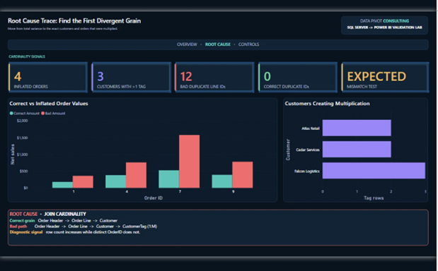
Figure 3: Power BI Root Cause Trace

The row inflation is restricted to four orders and to customers who have multiple tag rows.

The strongest signal is not how large the final total is. It’s the mix of signals: 18 rows become 28, distinct orders remain at 9, only 4 orders change value and the customers affected are those with multiple tag records. It is hard to explain that pattern as a DAX bug.

A practical reconciliation query can make the comparison formal:

SELECT
    OrderID,
    SUM(CorrectAmount) AS CorrectAmount,
    SUM(CandidateAmount) AS CandidateAmount,
    SUM(CandidateAmount) – SUM(CorrectAmount) AS Variance
FROM <order_level_reconciliation>
GROUP BY OrderID
HAVING SUM(CandidateAmount) <> SUM(CorrectAmount);

In production, the exact implementation might be two CTEs, temp tables, views or persisted validation tables. The main idea is to compare on a meaningful business key, not just on the final grand total.

Do the same for duplicates. The validated bad path has 12 duplicate line IDs, while the correct path has none. This is a real failure of the grain, not a formatting error.

Don’t succumb to the temptation to ‘fix’ the overstatement by dividing amounts by the number of tags, wrapping each measure in DISTINCT logic or creating a SUMX expression that attempts to re-create the intended grain inside DAX. Those techniques may produce a seemingly correct total for one report page but a different error under another filter. They also cause the semantic model to fix a source-shaping error that it did not introduce.

Validate Power BI Layer by Layer

Once the SQL Server result is correct, trace the data through Power BI in the order it moves through the system.

Your starting point is Power Query. SQL has the same rules concerning periods and status. If the query is on a relational source, query folding can be valuable as supported transformations can be pushed back to SQL Server. When performance matters, Microsoft recommends that you delegate as much relational processing to the source as practical, and check the step that breaks folding. Query folding is mostly a performance optimization, but it’s not a replacement for reconciliation. A quick query at the wrong grain is still wrong. 

Then look at the semantic model. Verify that the fact table still contains one row per OrderLineID. Look at the cardinality of the relationship and the filter direction. If CustomerTag is truly multi-valued, then model that relationship explicitly instead of hiding the multiplicity in the fact query. Microsoft’s guidance around relationship modeling indicates that the default is to filter in one direction and that many-to-many scenarios should be modeled deliberately rather than created as casual direct relationships.

Then deliberately make the first DAX measures boring:

Net Sales =
SUM ( SalesLine[NetSales] )
Order Count =
DISTINCTCOUNT ( SalesLine[OrderID] )
Line Count = COUNTROWS ( SalesLine )

These are sample names; adapt them to the model. The principle matters more than the syntax. If the table has duplicate fact rows, a simple SUM will return $4,825 and changing it to a more complex measure will not fix the data contract.

Finally, visually compare to the same SQL baseline. Here’s the dashboard we used: $2,830 source net sales, $4,830 bad-view net sales, $2,000 variance, 70.8% variance and 10 rows of inflation. It also identifies the affected orders and the customers causing the multiplication. The visualization is the end of the evidence chain, not the beginning of reconciliation.

It also saves you from another common anti-pattern, which is simply matching the total. The demo’s repeated-grain control is $5,650, or double the real $2,825. That number should alert a developer to a duplicate join right away, but whether to release should be a decision on the row/key/amount contract, not an intuition about the multiple.

Release Checklist, Practical Takeaways & Next Steps

If the source and report agree on the reporting window, grain, distinct business keys and additive measures, and any intentionally bad control throws the expected failure, the reconciliation process is ready to be released.

The contract accepted for this demo is simple: Jan-Feb 2026 is a half-open period ending before March 1, completed orders only, one row per OrderLineID, 18 correct rows, 9 orders, 6 customers, $2,825 net sales. The deliberately bad one-to-many path will fail with 28 rows and $4,825. The $2,000 overstatement is not something to be ‘corrected’ in the measure. It shows that the validation process can find a grain defect.

The workflow scales beyond this small data set. The same triplet can be stored in automated validation tables, checked on refresh and sliced by month, business unit, account, customer or another stable key on a large model. The idea is to keep the reconciliation near the grain, where the first divergence is explicable.

The best habit is to ask a new first question. Instead of asking, “What’s wrong with this DAX measure?” ask, “At what layer did the row count, distinct keys or additive amount first differ from the source contract?”

That alters the course of troubleshooting. This moves the investigation upstream, where the flaw is usually easier to identify and safer to fix. This allows DAX to do what it was designed to do: Calculate business logic on top of a trusted semantic model, not hide duplicated or inconsistently filtered source rows.